Table of regular polyhedra

22 Sep 2026

The five Platonic solids are well-known examples of regular polyhedra. Indeed, these are the only regular polyhedra in Euclidean 3D space if one requires that a polyhedron (1) be finite, (2) have planar faces, and (3) not intersect itself. However, if one relaxes all three of these restrictions, there are no longer 5 regular polyhedra but 48. Formally, we define a notion of “abstract regular polyhedron” (whose vertices, edges, and faces are not actual points or lines in space but merely elements of sets) and then consider all faithful discrete realizations of abstract regular polyhedra in Euclidean 3D space. The classification was first completed by Andreas Dress in a two-part 1985 paper called “A combinatorial theory of Grünbaum’s new regular polyhedra”. However, I have mostly based my tables on a later 1997 paper called “Regular polytopes in ordinary space” by P. McMullen and E. Schulte. I first became interested in this topic when I saw this Youtube video six years ago, but didn’t read McMullen and Schulte’s paper until earlier this month.

Of the 48 regular polyhedra, 18 are “blended” in the sense that there is a plane in 3D space that is never rotated by any symmetry of the polyhedron (but can be translated). The 30 non-blended polyhedra are listed in the table below.

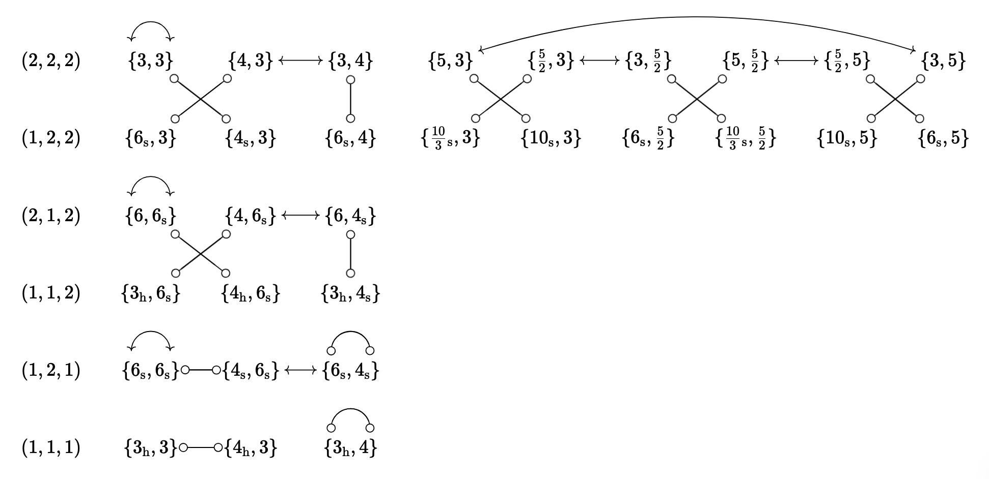
The symbol \(\{p,q\}\) denotes a polyhedron with faces of type \(\{p\}\) and vertex figures of type \(\{q\}\). The “vertex figure” of a polyhedron is the polygon formed by the vertices adjacent to a chosen vertex \(v\), where we draw a line between \(u\) and \(w\) if the edge connecting \(u\) to \(v\) and the edge connecting \(w\) to \(v\) are edges of the same face. A whole number without any subscript denotes a regular planar polygon with that many vertices. Thus, for example, \(\{3\}\) denotes a triangle, and \(\{3,4\}\) denotes a regular polyhedron whose faces are triangles and where each vertex has 4 coplanar vertices adjacent to it. (This is the octahedron.) A subscript “s” denotes a regular skew polygon, whose vertices alternate between two parallel planes, while a subscript “h” denotes a regular polygonal helix, which has infinitely many vertices. (For example, \(\{3_\mathrm{h}\}\) refers to a triangular helix.) For the record, the “s” and “h” notation is my own; it is similar to Dress’s notation, except that Dress uses superscripts that specify the exact angles involved. The last notational convention that might need explanation is the use of fractional numbers: a fraction \(\{\frac{p}{r}\}\) denotes a star polygon with \(p\) vertices, where one goes around the circle \(r\) times when drawing the polygon. Thus \(\{\frac{5}{2}\}\) refers to the regular pentagram.

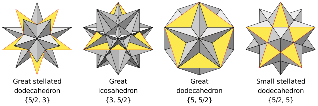
Some of the polyhedra in the table above are well-known. In particular, the first row contains the five platonic solids: the tetrahedron \(\{3,3\}\), the cube \(\{4,3\}\), the octahedron \(\{3,4\}\), the dodecahedron \(\{5,3\}\), and the icosahedron \(\{3,5\}\). The other four polyhedra in the first row are the “Kepler-Poinsot polyhedra”: the most common terms for these are (from left to right) the “great stellated dodecahedron”, the “great icosahedron”, the “great dodecahedron”, and the “small stellated dodecahedron”

The three polyhedra in the third row are known as the Petrie-Coxeter polyhedra and are distinguished by having planar faces but skew vertex figures. John Conway gave them the names “mutetrahedron”, “mucube”, and “muoctahedron”. All three were discovered in 1926: the mucube and the muoctahedron were discovered by Petrie, while the mutetrahedron was discovered by Coxeter shortly afterward. They extend infinitely in all three dimensions.

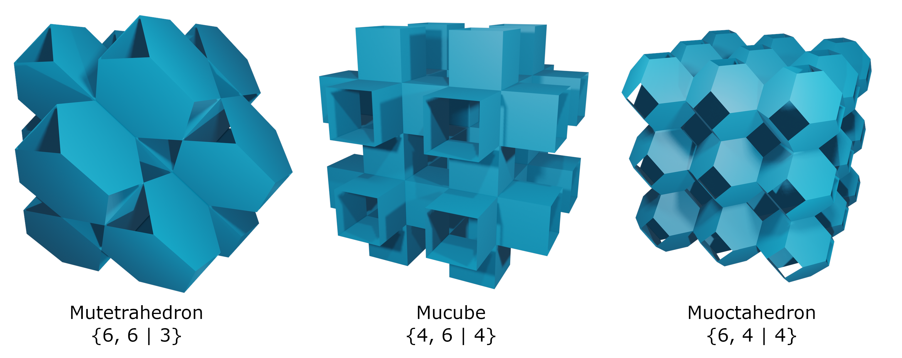
(Note: this image uses Coxeter’s original notation, which is also the notation used in McMullen and Schulte’s paper. The number after the vertical bar indicates the “holes” of the polyhedron. By the way, these renderings of the Petrie-Coxeter polyhedra as well as the Kepler-Poinsot polyhedra were taken from Wikipedia.)

Some features of my table of non-blended regular polyhedra remain to be explained. In particular, the triples of numbers on the left, along with the arrangement of rows and columns, provide information that allows one to generate any of the polyhedra in the table. The rules for generating a polyhedron \(P\) are as follows.

1. Look at the topmost polyhedron in the column containing \(P\). This will be a pair of numbers without any subscripts, say \(\{p,q\}\).

2. Create three planes \(A_0, A_1, A_2\), all passing through the origin in 3D space, such that the angle between \(A_0\) and \(A_1\) is \(\frac{\pi}{p}\), the angle between \(A_1\) and \(A_2\) is \(\frac{\pi}{q}\), and the angle between \(A_0\) and \(A_2\) is \(\frac{\pi}{2}\) (a right angle). Following McMullen and Schulte, I will use the same symbol for an affine subspace and the reflection through that subspace; I will also write composition in left-to-right order. Thus, for example, \(A_0A_1\) denotes reflection through \(A_0\) followed by reflection through \(A_1\); this is a rotation by \(2\pi/p\) radians around the line \(A_0\cap A_1\).

3. Look at the triple of numbers that begins the row of \(P\); call them \((d_0, d_1, d_2)\).

4. For each \(i\) from 0 to 2, define \(B_i\) as either \(A_i\) (if \(d_i = 2\)) or the orthogonal complement of \(A_i\) (if \(d_i = 1\)). Note that the dimension of \(B_i\) is \(d_i\). Note also that taking the orthogonal complement of a subspace corresponds to negating a reflection matrix.

5. If \((d_1, d_2) \neq (2, 2)\), or equivalently, if \(B_1 \cap B_2\) is merely a point (the origin) rather than a line, let \(C_0\) be a translation of \(B_0\) which still intersects \(B_2\). There is only ever one degree of freedom in choosing \(C_0\). In particular, in the case where \(B_0\) is a line and \(B_2\) is a plane, then \(B_0\) is in fact contained in \(B_2\) (since \(A_0\) is orthogonal to \(A_2\)). If \((d_1,d_2) = (2,2)\), we simply let \(C_0 = B_0\). In any case, we let \(C_1 = B_1\) and \(C_2 = B_2\).

6. If \((d_1, d_2) \neq (2, 2)\), then let \(F_0\) be the origin, and if \((d_1, d_2) = (2,2)\), then let \(F_0\) be a point that is not the origin but is contained in the line \(C_1 \cap C_2\). In both cases, we have \(F_0 \in (C_1 \cap C_2) \smallsetminus C_0\).

7. Let \(F_2\) be the polygon obtained by repeatedly applying \(C_0C_1\) and its inverse to \(F_0\). That is, \(F_2\) has edges

   \[\cdots - F_0(C_0C_1)^2 - F_0C_0C_1 - F_0 - F_0C_1C_0 - F_0(C_1C_0)^2 - \cdots.\]

   Let \(F_1\) be the edge from \(F_0\) to \(F_0C_1C_0 = F_0C_0\). Note that \(F_0C_0 \neq F_0\), so \(F_1\) (hence every edge of \(F_2\)) is nondegenerate. We call \(F_0, F_1, F_2\) the “initial” vertex, edge, and face of \(P\).

8. The other faces of \(P\) (and along with them, the other vertices and edges) can be obtained from \(F_2\) by applying combinations of \(C_0, C_1, C_2\).

Some remarks:

• The reflections \(C_0, C_1, C_2\) generate the symmetry group of \(P\). They have the property that \(C_i\) fixes \(F_j\) if and only if \(i \neq j\).

• When \(d_0 = d_1\), the angle between \(B_0\) and \(B_1\) is \(\frac{\pi}{p}\), and \(B_0B_1\) is a rotation of order \(p\). If \(d_0 = d_1 = 2\), then \(C_0C_1 = B_0B_1\), and \(F_2\) is a finite planar polygon \(\{p\}\). However, if \(d_0 = d_1 = 1\), then \(C_0C_1\) is a combination of \(B_0B_1\) plus a translation, and \(F_2\) is a helix \(\{p_\mathrm{h}\}\). This explains the positions of the “h”s in the table, and why the numbers subscripted with “h” always match the corresponding number in the first row.

• When \(d_0 \neq d_1\), the angle between \(B_0\) and \(B_1\) is \(\frac{\pi}{2} - \frac{\pi}{p}\), and \(B_0B_1\) (as well as \(C_0C_1\)) is a rotoreflection of order \(p'\) where \(\frac{1}{p} + \frac{1}{p'} = \frac{1}{2}\). If \((d_0, d_1) = (1, 2)\), then \(F_0\) is not on the mirror of \(C_0C_1\), and thus \(F_2\) is a skew polygon \(\{p'_\mathrm{s}\}\). If \((d_0, d_1) = (2, 1)\), then \(F_0\) is on the mirror of \(C_0C_1\), and thus \(F_2\) is a planar polygon \(\{p'\}\). This explains the alternation in the table between 3 and 6, 4 and 4, 5 and \(\frac{10}{3}\), and \(\frac{5}{2}\) and 10, when one looks at the face type of each polyhedron in a given column, and also explains why skew faces occur in rows 2 and 5.

• The vertex figure of \(P\) is generated by \(F_0C_0\) under the transformation \(C_1C_2\). When \(d_1 = d_2\), this transformation is a rotation of order \(q\), and we get a planar vertex figure \(\{q\}\). However, when \(d_1 \neq d_2\), this transformation is a rotoreflection of order \(q'\) where \(\frac{1}{q} + \frac{1}{q'} = \frac{1}{2}\) (with \(F_0C_0\) not on the mirror), and we get a skew vertex figure \(\{q'_\mathrm{s}\}\). This explains the alternation between different vertex figure types in the first three columns of the table.

• \(P\) is finite if and only if \(C_0, C_1, C_2\) have a common intersection. This happens if and only if we do not translate \(B_0\) to get \(C_0\); that is, if and only if \((d_1,d_2) = (2,2)\). In other words, the polyhedra in the first two rows are finite, and the polyhedra in the other four rows are infinite.

• If any of \(d_0,d_1,d_2\) are 2, then \(P\) has orientation-reversing symmetries and is achiral. However, if \((d_0,d_1,d_2) = (1,1,1)\), then \(P\) has no orientation-reversing symmetries and is chiral. The chiral polyhedra on row 6 of the table have helical faces which are all of the same handedness. (McMullen and Schulte give a nice description of the polyhedron which I denote \(\{4_\mathrm{h}, 3\}\) and which they denote \(\{\infty, 3\}^{(b)}\); its square helical faces run in three different directions.)

The last feature of the table that remains to be explained is the lines connecting some of the polyhedra. The double-headed arrows indicate duals; for instance, the octahedron is the dual of the cube. One can generate the dual of a polyhedron by replacing the mirrors \((C_0, C_1, C_2)\) with \((C_2, C_1, C_0)\), which interchanges the face and the vertex figure (modulo skewness). Only the polyhedra in the odd-numbered rows have duals.

The lines with circles at both ends indicate Petrie duals or “petrials”. The petrial of a polyhedron \(P\) has the same vertices and edges as \(P\) but different faces. Specifically, the faces of the petrial have the property that every two consecutive edges belong to a face of \(P\), but no three consecutive edges do. For example, the petrial of the cube, listed in the table as \(\{6_\mathrm{s},3\}\), has skew hexagonal faces which can be found by traversing the edges of the cube, turning left and right alternately at each vertex. All of the polyhedra in the table have petrials, with two being self-petrial.

We now come to the 18 blended polyhedra, which are listed in the table below. All are based on the three familiar tilings of the plane: the square tiling \(\{4,4\}\), the hexagonal tiling \(\{6,3\}\), and the triangular tiling \(\{3,6\}\).

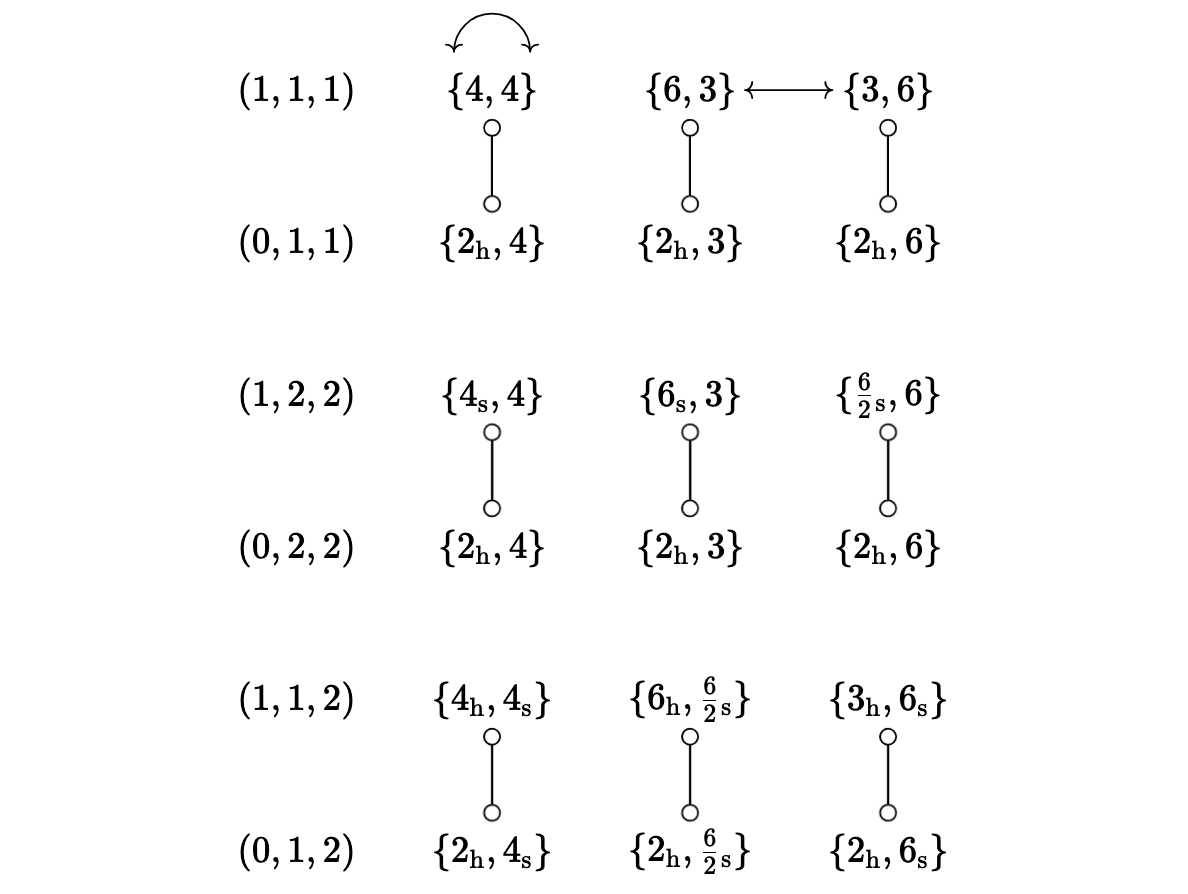
As in the table of non-blended polyhedra, the symbol \(\{p,q\}\) denotes a polyhedron with faces of type \(\{p\}\) and vertex figures of type \(\{q\}\). The symbol \(\{2_\mathrm{h}\}\) denotes an infinite planar zigzag, which can be thought of as a special case of a helix. The symbol \(\{\frac{6}{2}{}_\mathrm{s}\}\) denotes a skew six-sided polygon that wraps around the circle twice, forming a “skew triangle”.

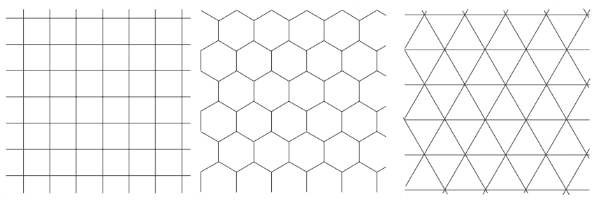
The polyhedra in the first row are simply the three regular planar tilings (depicted below). Note that the square tiling is self-dual while the hexagonal and triangular tilings are dual to each other, as indicated by the arrows in the table.

The polyhedra in the third row are “spiky” versions of the planar tilings. For the square and hexagonal tilings, the spiky version is constructed by lifting half of the vertices up to a higher plane, resulting in faces of type \(\{4_\mathrm{s}\}\) and \(\{6_\mathrm{s}\}\) respectively. For the triangular tiling, it is constructed by replacing each vertex with two vertices (lying on two parallel planes) and replacing each edge with two edges in a “X” configuration; the resulting faces are of type \(\{\frac{6}{2}{}_\mathrm{s}\}\).

The polyhedra in the fifth row are “helical” versions of the planar tilings. For the square and triangular tilings, the helical version is constructed by replacing each face by a helix; each helix has the opposite handedness compared to its neighboring helices. For the hexagonal tiling, we replace each face by two helices, one left-handed and one right-handed; this results in a vertex figure of type \(\{\frac{6}{2}{}_\mathrm{s}\}\).

The polyhedra in the even-numbered rows are simply the petrials of the ones above them, as indicated by the circle-ended lines. All have faces of type \(\{2_\mathrm{h}\}\). Arguably, my notation is not optimal in that it does not distinguish between all of the polyhedra, specifically the ones in row 2 and row 4, but the petrial lines make it clear which is which.

I should mention that the blended polyhedra in rows 3 through 6 (unlike the rest of the 48 polyhedra) are not actually single similarity classes, but infinite families related by stretching along a particular dimension. That is, the spiky tilings can be arbitrarily spiky, and the helices in the helical tilings can be arbitrarily stretched out.

Lastly, the triples of numbers on the left are the dimensions of the mirrors \((C_0,C_1,C_2)\) that (along with an initial vertex) generate a polyhedron in that row. Unlike in the table of non-blended polyhedra, the mirrors for different polyhedra in the same column are not related by taking the orthogonal complement; they are instead related in other ways. One can derive the mirrors \((C_0,C_1,C_2)\) from the polyhedron itself by taking an initial vertex, edge, and face \(F_0\subset F_1\subset F_2\), and then letting \(C_i\) be a symmetry of the polyhedron that fixes \(F_j\) if and only if \(i\neq j\). For the planar polyhedra (i.e. those in rows 1 and 2), the dimensions of the mirrors are not uniquely determined if one imagines the polyhedron as sitting in 3D space; I have used the lowest values, so that the mirrors are contained in the same plane as the polyhedron.